Looking at MCMC chains#
In this tutorial we will first generate chains for a simple model from the cobaya quickstart guide.
info = {
    "likelihood": {
        "gaussian_mixture": {
            "means": [0.2, 0],
            "covs": [[0.1, 0.05], [0.05, 0.2]],
        }
    },
    "params": {
        "a": {"prior": {"min": -0.5, "max": 3}, "latex": r"\alpha"},
        "b": {
            "prior": {"dist": "norm", "loc": 0, "scale": 1},
            "ref": 0,
            "proposal": 0.5,
            "latex": r"\beta",
        },
    },
    "sampler": {"mcmc": None},
    "output": "chains/mcmc",
}
from cobaya.yaml import yaml_dump_file

yaml_dump_file("gaussian_mixture.yml", info, error_if_exists=False)
Running the cobaya Monte-Carlo Markov Chains (MCMC) sampler will be pretty fast for such simple example.
from cobaya.run import run

updated_info, sampler = run(info)
We can now investigate how the parameters a and b for this Gaussian mixture likelihood have evolved. We first set the plot aesthetics via the set_style function from cobaya_utilities.plots module. By default, cobaya_utilities uses seaborn colors and theme scheme but you can get back to default matplotlib style by setting use_seaborn=False
from cobaya_utilities import plots

plots.set_style()
The cobaya_utilities.tools module allows to plot chains variation over MCMC steps.
from cobaya_utilities import tools

mcmc_samples = {"Gaussian mixture": "chains"}
params = ["a", "b"]
tools.plot_chains(mcmc_samples, params, ncol=1);
[root] *WARNING* outlier fraction 0.07857142857142857
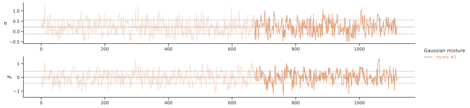
The plot_chains function takes a python dictionary holding the name of the MCMC and the path location to MCMC chains. You can select which sampled parameters you want to show and you can also tweak the figure layout (here the number of columns is set to 1). The gray lines represent the mean value (solid line) and the standard deviation (dashed lines) of the parameters for the full data chain. The shaded part of the chain corresponds to a typical 40% burnin but can be changed with the highlight_burnin parameters (default to 0.4).
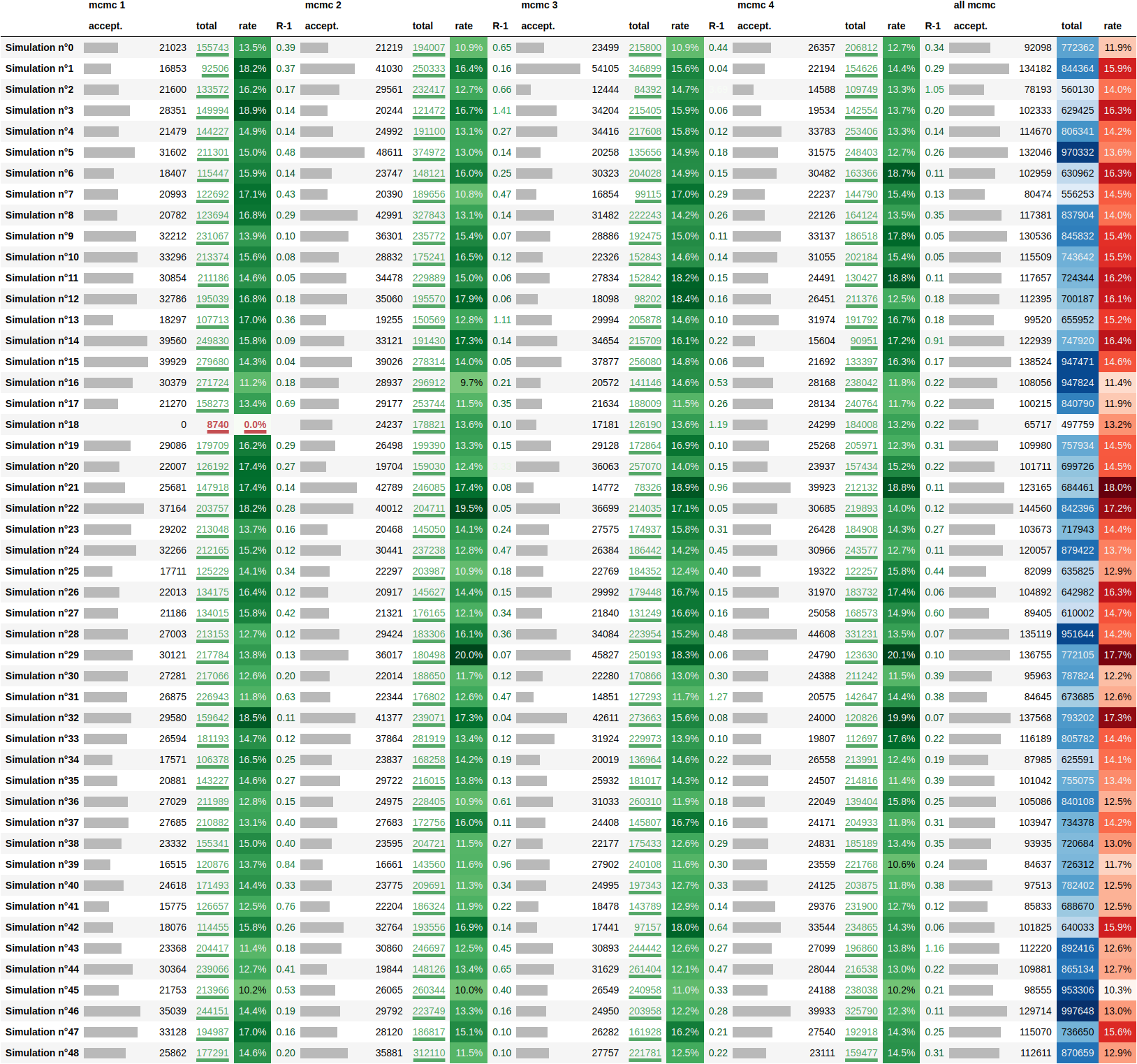
You can also plot the chain progress in terms of acceptance rate and Gelman \(R-1\) parameter (as reminder cobaya already provides such monitoring tool but we will see later how, in special running, the plot_chains function is more versatile to the default cobaya’s one)
tools.plot_progress(mcmc_samples);

We can finally print the mean and \(\sigma\) values extracted from getdist and showed in a pandas Dataframe
from getdist.plots import loadMCSamples

tools.print_results(
    [loadMCSamples(f"{path}/mcmc") for path in mcmc_samples.values()],
    params=params,
    labels=mcmc_samples,
)
| $\alpha$ | $\beta$ | |
|---|---|---|
| Gaussian mixture | $ 0.20^{+0.32}_{-0.37}$ | $ 0.03\pm 0.41$ |
Running several MCMC chains#
In the most common use case, MCMC are run in cluster machines and the usual way is to run several chains with different starting points in parallel. If you have mpi installed you can follow the cobaya guide. If you have no access or a limited one to mpi machines (for instance, CC-IN2P3 cluster has poor support for mpi jobs), you can run separate and independant chains as follow
%%bash
rm -rf chains/*
for i in {1..4}; do
    cobaya-run -o chains/mcmc.${i} gaussian_mixture.yml > chains/mcmc.${i}.log
done
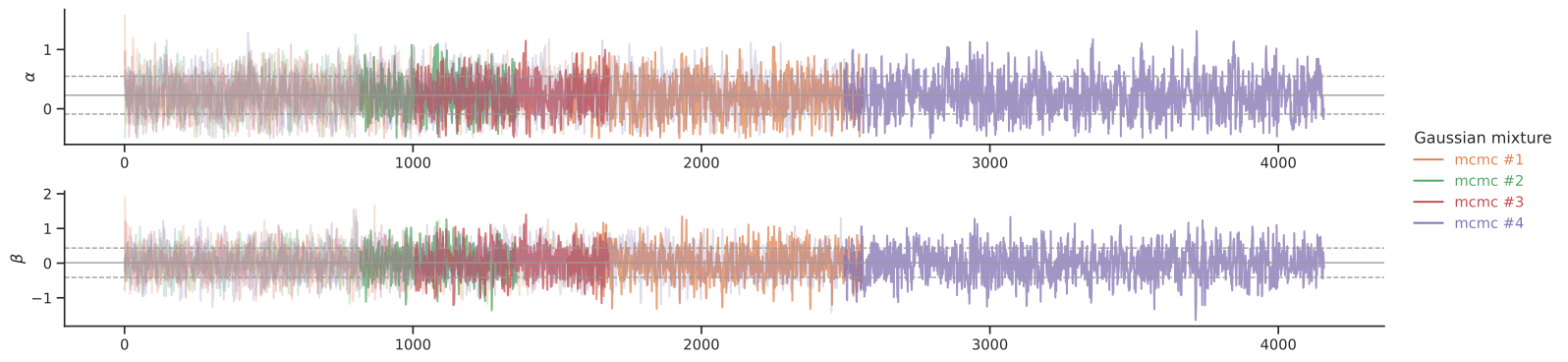
with the resulting plots
tools.plot_chains(mcmc_samples, params, ncol=1);
Create MCMC symlinks...
[root] *WARNING* outlier fraction 0.00390625
[root] *WARNING* outlier fraction 0.04632352941176471
[root] *WARNING* outlier fraction 0.025595238095238095
[root] *WARNING* outlier fraction 0.0002403846153846154
tools.plot_progress(mcmc_samples);

Finally, for getting some statistics of the different MCMC, cobaya_utilities provides a function named print_chains_size which return a pandas Dataframe with different informations such as the accepted and total steps, the corresponding rate and \(R-1\) value. The print_chains_size function actually parsed the logfile mcmc.?.log which stores the printed output from cobaya-run execution. For such simple example, there is not a lot to learn since the convergence is almost immediate but, for longer MCMC runs (see below), this is another way to monitor your MCMC flow.